findings - analog devices

INTRODUCTION
When a process is controlled (Figure 1), a characteristic of the process, such as a temperature (regulated variable), is compared with the desired value, or setpoint. The difference, or error signal, e(t), is applied to a controller, which uses the error signal to produce a control signal, u(t), that manipulates a physical input to the process (manipulated variable), causing a change in the regulated variable that will stably reduce the error.

A commonly used control operator is a proportional-integral-derivative (P-I-D, or PID) controller. It sums three terms derived from the error: a simple gain, or proportional term; a term proportional to the integral of the error, or integral term; and a term proportional to the rate of change of the error signal, or derivative term. In the closed loop, the proportional term seeks to reduce the error in proportion to its instantaneous value; the integral term - accumulating error - slowly drives the error towards zero (and its stored error tends to drive it beyond zero); and the derivative term uses the rate of change of error to anticipate its future value, speeding up the response to the proportional term and tending to improve loop stability by compensating for the integral term’s lag.

The combination of these terms can provide very accurate and stable control. But the control terms must be individually adjusted or “tuned” for optimum behaviour in a particular system. Because processes with many lags or substantially delayed response are hard to control, a simple PID controller is best used for processes that react readily to changes in the manipulated variable (which often controls the amount or rate-of-flow of energy added to the process). PID control is useful in systems where the load is continually varying and the controller is expected to respond automatically to frequent changes in setpoint—or deviations of the regulated variable (due to changes in ambient conditions and loading)

Fig1
Figure 1. Control loop employing a PID control function

The parameters of PID controllers for slow processes are usually obtained initially by working with system models scaled up in speed. There are many advanced control strategies, but the great majority of industrial control systems use PID controllers because they are standard, time-tested, well understood industrial components. Moreover, due to process uncertainties, a more-sophisticated control scheme is not necessarily more efficient than a well-tuned PID controller for a given process.

The PID terms were briefly explained above. Here is a more complete explanation of them.

Proportional Control
Proportional control applies a corrective term proportional to the error. The proportionality constant (Kp) is known as the proportional gain of the controller. As the gain is increased, the system responds faster to changes in setpoint, and the final (steady-state) error is smaller, but the system becomes less stable, because it is increasingly under-damped. Further increases in gain will result in overshoots, ringing, and ultimately, undamped oscillation.

Integral Control
Although proportional control can reduce error substantially, it cannot by itself reduce the error to zero. The error can, however, be reduced to zero by adding an integral term to the control function. An integrator in a closed loop must seek to hold its average input at zero (otherwise, its output would increase indefinitely, ending up in saturation or worse). The higher the integral gain constant, Ki, the sooner the error heads for zero (and beyond) in response to a change; so to set Ki too high is to invite oscillation and instability.

Derivative Control
Adding a derivative term—proportional to the time derivative, or rate-of-change, of the error signal—can improve the stability, reduce the overshoot that arises when proportional and/or integral terms are used at high gain, and improve response speed by anticipating changes in the error. Its gain, or the “damping constant,” Kd, can usually be adjusted to achieve a critically damped response to changes in the setpoint or the regulated variable. Too little damping, and the overshoot from proportional control may remain; too much damping may cause an unnecessarily slow response. The designer should also note that differentiators amplify high frequency noise appearing in the error signal.

In summary, a proportional controller (P) will reduce the rise time and will reduce, but never eliminate, the steady state error. A proportional-integral (PI) controller will eliminate the steady state error, but it may make the transient response worse. A proportional-integral-derivative controller (PID) will increase the system stability, reduce the overshoot, and improve the transient response. Effects of increasing a given term in a closed-loop system are summarized in Table I

The sum of the three terms is

The corresponding operational transfer function is:

In the system of Figure 1, the difference between the setpoint value and the actual output is represented by the error signal e(t). The error signal is applied to a PID controller, which computes the derivative and the integral of this error signal, applies the three coefficients, and performs the above summation to form the signal, u(t).

Digital PID Control
The PID algorithm, now widely used in industrial process control, has been recognized and employed for nearly a century, originally in pneumatic controllers. Electronics—first used to model PID controls in control-system design with analog computers in the 1940s and ’50s—became increasingly involved in actual process-control loops, first as analog controllers, and later as digital controllers. Software implementation of the PID algorithm with 8-bit microcontrollers is well documented.

In this article we show the basic components of a digital PID controller—and then show how process control can be implemented economically using a MicroConverter®, a data-acquisition system on a chip.

One might consider the use of a PID loop, for example, in an air conditioning or refrigeration system to accurately maintain temperature in a narrow range, using continuous monitoring and control (as opposed to thermostatic on-off control). Figure 2 shows a basic block diagram of a control system that regulates temperature by continuously adjusting fan speed, increasing or decreasing the airflow from a low-temperature source.

Figure 2. Example of a PID controller for a temperature-controlled ventilation system using discrete components.

The system is required to maintain the room temperature as close as possible to the user-selected (setpoint) value. To do this, the system must accurately measure the room temperature and adjust the fan speed to compensate.

In the system shown in Figure 2, a precision current source drives a current through a resistive temperature sensor—a thermistor or RTD—in series with a reference resistor, adjusted to represent the desired temperature. The analog-to-digital converter (ADC) digitizes the difference between the reference voltage and the thermistor voltage as a measure of the temperature error. An 8-bit microcontroller is used to process the ADC results, and to implement the PID controller. The microcontroller adjusts the fan speed, driving it via the digital-to-analog converter (DAC). External program memory and RAM are required to operate the 8-bit microcontroller and execute the program.

If proportional control (P) on its own were used, the rate at which the fans run would be directly related to the temperature difference from the setpoint. As mentioned earlier, this will leave a steady state error in place.

Adding an integral term (PI) results in the fan speed rising or falling with the ambient temperature. It adjusts the room temperature to compensate for errors due to the ambient rise in temperature through the day and then the temperature fall in the evening. The integral term thus removes the offset, but if the integral gain is too high, oscillation about the setpoint can be introduced. (Note that oscillation is inherent in temperature-control systems employing on-off thermostats.)

This oscillatory tendency can be greatly reduced by adding in a derivative term (PID). The derivative term responds to the rate of change of the error from the setpoint. It helps the system rapidly correct for sudden changes due to a door or window being opened momentarily.

To simplify this system, minimizing parts cost, assembly cost, and board area, an integrated system-on-a-chip (SOC) solution can be used, as shown in Figure 3.

Figure 3. System-on-a-chip implementation.

The ADuC845 MicroConverter includes 62K bytes of flash/EE program memory, 4K bytes of flash data memory, and 2K bytes of RAM. The flash data memory can be used to store the coefficients for a ‘tuned’ PID loop, while the single-cycle core provides enough processing power to simultaneously implement the PID loop and perform general tasks.

Depending on which MicroConverter is selected, the resolution of the ADC ranges from 12 to 24 bits. In a system where the temperature needs to be maintained to 0.1°C accuracy, the ADuC845’s high performance 24-bit sigma-delta ADC is ideal.

A second type of application where a PID control loop is useful is setpoint (servo) motor control. In this application the motor is required to move to, maintain, and follow an angular position defined by a user input (for example, the rotation of a potentiometer—Figure 4).

Figure 4. Example of a motor control system embodied with discrete components.

Again, this system can be implemented using many discrete components or, more simply, with an integrated solution. Figure 5 shows a demonstration system built using the MicroConverter. The circuitry on the board causes the pointer to follow the rotation of the setpoint input potentiometer.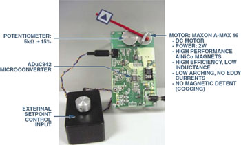

Figure 5. Sample motor control system using discrete components.

Figure 6. System-on-a-chip implementation of Figure 4.

With the blocks integrated in the compact form of the ADuC842, parts and assembly costs are lower; the computational electronics occupies considerably less space and is more reliable. Figure 6 shows the simplicity of the system hardware using the SOC approach.

Besides the ADuC842, the board includes a potentiometer buffer amplifier, an output power amplifier that drives the motor, a 5-V low-noise regulator for the low-power electronics, and a huskier 5-V regulator (with heatsink) for the motor. The board also includes status LEDs, a RESET button, a serial-data download button, and some passive elements.Using PC software to simulate the rest of the system, Figure 7 shows responses for different levels of system tuning, and demonstrates the importance of the integral term.

Figure 7. Proportional-integral (P-I) control for three settings of the integral term.
Note the offset from 1.0 for KI = 0, the lightly damped oscillatory tendency for KI = 2000, with oscillations almost eliminated at KI = 550.

The improvement in overall system step response when implemented with the full PID loop is clearly shown in Figure 8. The response is fast, accurate, and damped, with no offset, oscillation, or overshoot.

Figure 8. Proportional-integral-derivative (PID) control response.

This articles was written by Eamon Neary [eamon.neary@analog.com] from Analog Devices - www.analog.com